Breast Cancer Detection using Deep Learning – speeding up histopathology

Introduction – We do live in a better world

A great number of voices claim that the world is in a terrible shape and that an apocalyptic future awaits us. The truth is that life has never been better. We live in a world in which extreme poverty has dropped from 30 percent in 1990 to 10 percent in 2015 (Globalization’s great triumph: The death of extreme poverty), meaning that, given the increase in population during that period, 130 000 a day (A DAY!!!!) have broken free from extreme poverty. This has been achieved faster than anyone could have dreamed of. Advances in technology, agriculture, housing, energy storage and manufacturing, together with a more transparent global society have put an end to a lot of the suffering inflicted upon billions and thereby ended a multitude of conflicts. The rise of AI is a promise of even greater human achievements. There are issues, both moral and ethical ones, that need to be dealt with, but for the time being we are far from the gloomy prospect of being enslaved by some malevolent general AI and we should use this ”new” technology for a greater good.

One of the many areas in which AI has a potential to elevate us even higher is medicine. Medical advances and availability to them have saved hundreds of millions from unnecessary suffering and death. So, yes we do live in a far better world than many think…and it just keeps getting better. We now have the ability to, at very low costs, store terabytes upon terabytes of data, from journals, books, sounds and images. We know how to develop AI models to detect objects, masses or anomalies and these models cost nothing to create in comparison to the costs spent on the time of specialized professionals going through files and images, day after day, year in and year out. The costs are particularly problematic for individuals living in parts of the world which still have low incomes and for whom serious illnesses can be devastating, not only for the individual but for entire families.

In this blog post, I revisit a previous post I wrote a while ago in which I presented a data format used in medicine, the DICOM-format (click link to see post). The DICOM-format enables the gathering of all patient info and x-ray images to ensure that the two sets of information can never be separated and thereby reduce the risk of mismatch. I focused on mamogram and had the intention of writing a sequel to the post in which I trained a model to identify cancer cases in mamograms. Unfortunately, the format of these images (lossless jpeg) is obsolete and I haven’t been able to use them in a satisfactory manner. Instead, I chose to use a dataset of prepared breast tissue slides made available on kaggle, The Breast Histopathology Images.

Note that this set back doesn’t mean I have abandoned the initial goal of training a model on mammograms. Not having this option for the moment does not mean that the technique cannot be used further down the treatment chain. As we point out in the next section, the incidence of breast cancer is the highest in Western and Scandinavian countries and the lowest in in Eastern and Central Africa, as well as in Eastern and South-Central Asia. Yet, the 5 year survival rate is the highest in Western and Scandinavian. This is due to the availability and cost of screening and histopathology, which has to be performed by highly skilled professional. AI thus has the potential to democratize medical processes and save millions of women (and men) from unnecessary and painful deaths.

 

Histopathology and getting enough data

Breast Cancer and Histopathology

Normally, when a professional suspects the presence of a tumor, the natural next step is to perform a biopsy to obtain a sample of the suspected tissues. This does not mean that the patient has cancer and even if there is a tumor, it might just be begnin. It still needs to be inspected. The act of doing this is called histopathology. Now, not everyone has had the advantage of studying greek in school, so the word Histopathology, might seem somewhat mysterious. Histopathology is the concatenation of three words histo, which means tissue, pathos, which means suffering (read disease) and logia which means study. Hence, histopathology is the study of diseased tissues.

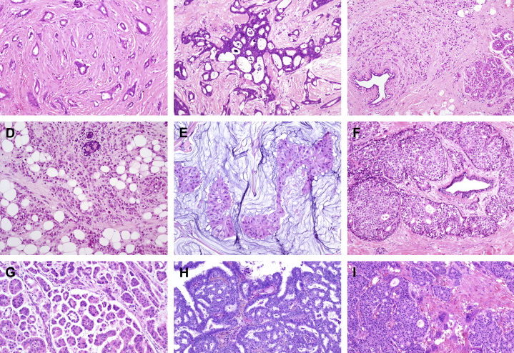
The samples are often colored with with hematoxylin and eosin. The staining method involves application of hemalum, a complex formed from aluminium ions and hematein (an oxidation product of hematoxylin). Hemalum colors nuclei of cells blue, along with a few other objects, such as keratohyalin granules and calcified material, which turns blue when exposed to alkaline water (blueing solution). The nuclear staining is followed by counterstaining with an aqueous or alcoholic solution of eosin Y, which colors eosinophilic structures in various shades of red, pink, and orange. (source: wikipedia)

Figure 1: Hematoxylin and eosin breast tissue.

We will working with The Breat Histopathology Image dataset. It is a set of whole slide images of breast cancer for the detection of Invasive Ductal Carcinoma (IDC) or Infiltrating Ductal Carcinoma (IFD), which is the most common type of breast cancer (80 percent of all breast cancers). It is called ductal becasuse the cancer started in the conduct trasnporting milk from the milk-producing lobules to the nipples. The fact that it is called Invasive comes from the fact that it has spread to the surrounding breast tissue. Carcinoma means that the cancer started in skin or tissue that cover internal organs. The symptom vary but it is accepted that the following symptom may be the first sign of invasive ductal carcinoma: Swelling of all or part of the breast, skin irrtation or dimpling, pain, nipple pain, redness, scaliness or thickening of the niple, nipple discharge or a lump in the underarm areas.

Like most cancers, the earlier it is detected the better the chances for survival are. There are 4 stages of breast cancer and the 5 year survival rates for North American women are 100%, 93%, 72% and 22%, respectively. There are racial differences in the likelihood of developing breast cancer, which in turn influences the five year survival rate for different regions. Western women have for instance the highest risk of developing breast cancer while women in Eastern and Central Africa, as well as in Eastern and South-Central Asia, have the lowest incidence. The figure below shows however that an early detection is paramount to survival.

Figure 2: Breast Cancer five year survival ratte by country (Healthline.com)

 

The Breast Histopathology Image dataset Content and a slight problem

We mentioned above that the set of images that we will be working with is called the the Breat Histopathology Image dataset and that we obtained it from kaggle. it was originally created in an attempt to develop Deep Learning models and and compare their accuracy. (see: Automatic detection of invasive ductal carcinoma in whole slide images with Convolutional Neural Networks, Cruz-Roa et al.). Among the models used were Random Forest models and a Convolutional Neural Network. We are going to do something quite similar and compare our results with the ones previously obtained. Finally, we will end the post with a discussion on how to improve the results and why it is imperative that models of the sort be used globally.

The dataset was originally curated by Janowczyk and Madabhushi and Roa et al. and consists of 162 slide images scanned at 40x (i.e. 162 patient cases). Slide images are quite large so in order to make them easier to work with, a total of 277 524 patches were created from the original slides:

• 198 738 IDC negatives
• 78 786 IDC positive

As you notice, the number of IDC-negative cases is 2,5 times that of IDC-positive cases. And that can’t be good if your aim is to use the data in a neural network. Suppose that we do not address the problem, we risk some severe issues. Assume that we construct two models, Model X and Model Y, to classify histopathologies into the two available classes, IDC-negative and IDC-positive. Our two models perform in the following way:

• Model X classifies 8 out of 10 IDC-positive images as IDC-negatives and 10 out of 10 000 IDC-negatives as IDC-positives.
• Model Y classifies 1 out of 10 IDC-positive images as IDC-negatives and 100 out of 10 000 IDC-negatives as IDC-positives.

Model X thus makes 18 mistakes while Model Y makes 101 mistakes. Both are terrible and come with their own non-acceptable consequences. In any case, most machine learning models will pick Model X since in minimizes the total number of errors.  Dealing with this issues is dealt in the following section.

Class Imbalance and solutions

As we mentioned in the previous section, class imbalance, i.e. the fact that there are fewer examples of one category of pictures than the other, can create problems when training an AI model. There are basically four ways of dealing with the issue:

1. Introducing a cost function: If we think it is worse to identify a IDC-positive as an IDC-negative, the cost function ought to take that into account and count every such error as x such errors.
2. Sampling:

• Undersampling: To remove images from the majority class, in our case this would mean removing IDC-negative images. The problem that may occur with undersampling is the risk of removing really significant examples from the dataset. The impact is a drop in the accuracy of the model.
• Oversampling: To add more images from the minority class, which in our case would mean adding IDC-positive images. This would either be done by aquiring new images or by generating them. It might be hard to obtain new images (otherwise you might already have had them). The other option is generating these images from existing ones by changing the contrast, flipping images, croping the, rotating them and other methods. The problem is that you may not get the variety that you were hoping for and might just have created copies of your data.
• Under-Oversampling: A combination of under- and oversampling. The problem with this method combines the risks from both original methods.

How one chooses to deal with imbalance often depends on how large the imbalance is and on the problem that one is dealing with. But eliminating the imbalance is always a good thing. In the case of cancer detection, one wants to avoid preference for the dominating class, i.e. the IDC-negative class.

For this excerise, we chose to undersample the majority class and randomly removed images from the IDC-negative set of images. One can argue that this might be detrimental for modelling purposes, but the end result of our work is still a hybrid of over- an undersampling. Indeed, when the undersampling process is performed, we are left with fewer examples than we started with, which is not really a good result. A solution is then to augment the resulting dataset by generated new images through a series of geometric transformations such as isometries (rotations, flips, translations, magnifications). There are several ways of doing this. One of them is to generate these images by using generating function that can be written in Python:

import numpy as np

import os

from keras.preprocessing.image import ImageDataGenerator

from scipy import ndimage

 

image_path     = ’…..//kaggleSetResized’

save_here      = ’……//result’

samples_per_0  = 1        #the values can be changed if the datasets hasn’t been undersampled

samples_per_1  = 1        #the values can be changed if the datasets hasn’t been oversampled

indexfile_path = ’……//index.csv’

delimiter = ’,’

 

# Image generation function

datagen = ImageDataGenerator(rotation_range=10,

                             width_shift_range=0.1,

                             height_shift_range=0.1,

                             shear_range=0.15,

                             zoom_range=0.1,

                             channel_shift_range=10,

                             horizontal_flip=True)

 

 # Empty Target directory

for path, subdir, images in os.walk(save_here):

    for image in images:

        os.remove(path+’/’+image)

 

for path, subdir, images in os.walk(image_path):

    for image in images:

        parts = image.split(’class’)

        cat = parts[-1][0]

        prefix = parts[0]

        image = path+’/’+image

        save_here_cat = save_here+’/’+cat

        samples_per_image = samples_per_0

        if cat == ’1’:

            samples_per_image = samples_per_1

       

# Original image sampling

        image = np.expand_dims(ndimage.imread(image), 0)

 

# Fit original image

        datagen.fit(image)

 

# Iterate over images and save

        for x, val in zip(datagen.flow(image,                         

                                       save_to_dir=save_here_cat,    

                                       save_prefix=prefix,           

                                       save_format=’png’),

                                       range(samples_per_image)):    

            Pass

 

Alternatively, if one uses a platform such as Peltarion Operational AI Platform  one doesn’t need to do this step. One of the huge advantages is, besides not having to code anything, not having to allocate any disk space for the set of newly created images. Another advantage is that completely new images are created at every iteration, hence creating a true image augmentation.

 

Image augmentation in Peltarion

Filling empty spaces with different methods

 

What model to choose?

Since we are dealing with images, we know that convolutional neural networks (CNN) are good guesses for the job. But there is a multitude of potential CNN candicates more or less suited for the images that we are dealing with in this example.  For this example, I chose to test three different models, namely AlexNet, ResNet and DenseNet, to compare their ability to classify histopathologies of breast cancer. Before going into the results, let’s say something about these models and explain some of the ways in which they differ. For a description of AlexNet the reader should read Sopra Steria Analytics previous blog post, Using CNN for speech emotion recognition. Whats wrong with it?

 

Properties of ResNet and DenseNet

Because of the complexity of the images we feed our network, we need a rather deep network in order to properly do our job. It is however a known fact that the deeper a network is the greater the risk that too much information (input or gradient) gets lost as it passes the different layers for the model to be valuable.

A residual neural network builds on constructs known as pyramidal cells in the cerebral cortex. They do this by making use of so called skip connections to jump over a given number of layers in the network (at least one). The reason for skipping layers is the need to avoid vanishing gradients by reutilizing activations from layers upstream in the network until the layer next to the current one learns its weights. Skipping compresses the network into fewer layers, thereby speeding up the learning process. The skipped layers are then restored as the network learns the feature space. A special case of ResNet is the so called DenseNet, in which several parallel layer skips are performed.

Recent work has shown that CNNs can be deeper, without loss of information and thus more accurate as well as more efficient to train, if they contain connections between layers close to the input and those close to the output. Neural network of that type are called Dense Convolutional Network (DenseNet) and connect each layer to every other layer in a feed-forward fashion. Traditional CNN with L layers have L connections — one between each layer and its subsequent layer —  while DenseNet has L(L+1)/ 2 connections. The feature-maps of all layers are used as inputs to the next layer, and its own feature-maps are used as inputs into all subsequent layers. DenseNets have some really nice properties:

• Mitigates the problem of vanishing-gradients
• Pushes feature propagation
• Encourages feature recycling
• Reduces the number of parameters

Traditional feed-forward neural networks such as AlexNet and ResNet connect the output of each of their layers to the next layer. Normally this includes performing a convolution operation or pooling layers, a batch normalization and an activation function. For those who are not really sure of how this work, there are plenty of descriptions online or in one of my previous blog posts, A gentle introduction to Image Recognition by Convolutional Neural Network. In mathematical terms this amount to the following equation:

 

Another way of doing this is to skip connections and thus perform what a conventional CNN does augmented with a skipped information flow,

thus summing the output feature maps of the layer with the incoming layer. DenseNet does something different, it concatenates them,

One can immediately understand that information of the input is less likely to be lost. One drawback though is that it is much more demanding to use DenseNet and that the models take much more time to train.

 

Results and discussion

In our experiment we have tried three different network types, namely AlexNet, ResNet and DenseNet. The results vary slightly but reach approximately the same accuracy. I have gathered some of the key values to look at for the three models:

Now, it looks as if AlexNet reaches the highest precision, tightly followed by ResNet, but one needs to be careful when drawing conclusions. Look for instance at the  confusion matrices for the three model types below:

Recall that the IDC-negative images are labelled 0, with those being classified as exhibiting IDC are labelled 1. This means that we want as few false-negatives as possible, i.e., we do not want to claim that a patient does not have breast cancer when she/he actually does. Naturally, we also wish to have as few false-positives as possible but the consequences of false-negatives are worse than those of false-positives.

The scope of this blog post was mainly to show that it is a straightforward thing to actually design and train a model for cancer detection given that the data used is good enough. Ideally, one would wish to have more data, such as all the measurements made by physicians, about the patient (demographic variables, lifestyle etc.).

There are actually one things that we have not had the possibility to influence, namely the origin of the data. The 277 000+ images that we use in our models originate from 162 slides that have been cut into 50 pixels * 50 pixels patches. This raises a range of questions that in many ways cast a shadow on how well a model can be trained.

That being said, availability of more data from a greater number of patients certainly gives hope to obtain better results. Also, even though the accuracy is not sufficiently high to have an unsupervised automated classification one can most probably use a tool building on the ResNet model to assist physicians in simple cases. Indeed, the false-positive and false-negative case may be particularly hard to classify. Further work, in association with professionals may be required to explain to misclassification.